library(tidyverse)
library(rvest)
library(httr)
library(scales)
library(broom)
I was wondering what is the current price of my car on the market. One way how to get some at least bit objective value is based on current situation on the market. I´m about to use simple (yet effective) web scraping technique to retrieve data from local best known internet car marketplace.
First step - how many pages?
As a first step we need to find out on how many pages are the offers related to the same type of my car. By piping the root path to read_html and selecting node “a.hide-S”" we can find it out.
path <- "https://www.tipcars.com/skoda-rapid/benzin/"
# get max. page
max <- path %>%
  html_session() %>%
  read_html %>%
  html_nodes("a.hide-S") %>%
  html_text()
max
## [1] "8"..pages, each with 100 cars. Now you may ask how did I know which node to use? And an answer would be simple - using SelectorGadget tool. It is pretty cool tool allowing you to select any item on web page of your interest and provide “node” to it. You can find out how to use it here.
Load all URLs
Now we can use information about number of pages to create vector of sites we will scrape.
url <- paste0(path,"?str=",1:max, "-100")
url
## [1] "https://www.tipcars.com/skoda-rapid/benzin/?str=1-100"
## [2] "https://www.tipcars.com/skoda-rapid/benzin/?str=2-100"
## [3] "https://www.tipcars.com/skoda-rapid/benzin/?str=3-100"
## [4] "https://www.tipcars.com/skoda-rapid/benzin/?str=4-100"
## [5] "https://www.tipcars.com/skoda-rapid/benzin/?str=5-100"
## [6] "https://www.tipcars.com/skoda-rapid/benzin/?str=6-100"
## [7] "https://www.tipcars.com/skoda-rapid/benzin/?str=7-100"
## [8] "https://www.tipcars.com/skoda-rapid/benzin/?str=8-100"To get HTML structure of each page in list is map useful function.
html_list <- url %>%
  map(html_session) %>%
  map(read_html)
This simple function extracts text from defined node and html (both input parameters).
getText <- function(html, node) {
  html %>%
    html_nodes(node) %>%
    html_text(trim = TRUE) %>%
    as.tibble()
}
Map map map
# initiating df with extraction of car prize
df <- html_list %>% map(getText, ".fs-tluste") %>%  map(~.[2:nrow(.),]) %>% bind_rows()
## Warning: `as.tibble()` is deprecated, use `as_tibble()` (but mind the new semantics).
## This warning is displayed once per session.df <- df %>%
rename(cost = value) %>%
# extract engine
mutate(model = html_list %>% map(getText, ".motor") %>% unlist) %>%
# extract mileage
mutate(mileage = html_list %>% map(getText, ".najeto") %>% unlist) %>%
# extract year of production
mutate(year = html_list %>% map(getText, ".rok_vyroby") %>% unlist)
df## # A tibble: 772 x 4
## cost model mileage year
## <chr> <chr> <chr> <chr>
## 1 125 122 Kč benzin, 42 kW 39 tkm 1984
## 2 129 999 Kč benzin, 1 197 ccm, 63 kW 276 tkm 2014
## 3 134 400 Kč benzin, 1 197 ccm, 63 kW 119 tkm 2014
## 4 149 900 Kč benzin, 1 198 ccm, 55 kW 87 tkm 2013
## 5 155 000 Kč benzin, 1 197 ccm, 63 kW 153 tkm 2015
## 6 159 000 Kč benzin, 1 197 ccm, 63 kW 156 tkm 2014
## 7 159 000 Kč benzin, 1 197 ccm, 63 kW 132 tkm 2013
## 8 160 000 Kč benzin, 1 197 ccm, 63 kW 122 tkm 2013
## 9 164 000 Kč benzin, 1 197 ccm, 63 kW 102 tkm 2013
## 10 168 000 Kč benzin, 1 197 ccm, 66 kW 197 tkm 2015
## # ... with 762 more rowsHere we have cars of interest (all Škoda Rapid gasoline variants). Let´s decompose it more using a bit of regular expression.
final <- df %>%
  # select numbers only
  mutate(cost = str_extract(cost, "^[0-9]+ [0-9]+")) %>%
  # replace white space
  mutate(cost = str_replace_all(cost, "\\p{WHITE_SPACE}", "")) %>%
  # conversion to double
  mutate(cost = cost %>% as.numeric()) %>%
  # extract power
  mutate(kW = str_extract(model, "[0-9]{2} kW")) %>%
  # get rid off "kW"
  mutate(kW = str_extract(kW, "[0-9]{2}")) %>%
  # conversion to factor
  mutate(kW = kW %>% as.factor()) %>%
  # extract mileage
  mutate(mileage = str_extract(mileage, "^[0-9]+")) %>%
  # conversion to double
  mutate(mileage = mileage %>% as.numeric() * 1000) %>%
  select(model, mileage, cost, kW, year)
final
## # A tibble: 772 x 5
## model mileage cost kW year
## <chr> <dbl> <dbl> <fct> <chr>
## 1 benzin, 42 kW 39000 125122 42 1984
## 2 benzin, 1 197 ccm, 63 kW 276000 129999 63 2014
## 3 benzin, 1 197 ccm, 63 kW 119000 134400 63 2014
## 4 benzin, 1 198 ccm, 55 kW 87000 149900 55 2013
## 5 benzin, 1 197 ccm, 63 kW 153000 155000 63 2015
## 6 benzin, 1 197 ccm, 63 kW 156000 159000 63 2014
## 7 benzin, 1 197 ccm, 63 kW 132000 159000 63 2013
## 8 benzin, 1 197 ccm, 63 kW 122000 160000 63 2013
## 9 benzin, 1 197 ccm, 63 kW 102000 164000 63 2013
## 10 benzin, 1 197 ccm, 66 kW 197000 168000 66 2015
## # ... with 762 more rowsNow the data are ready to be plotted.
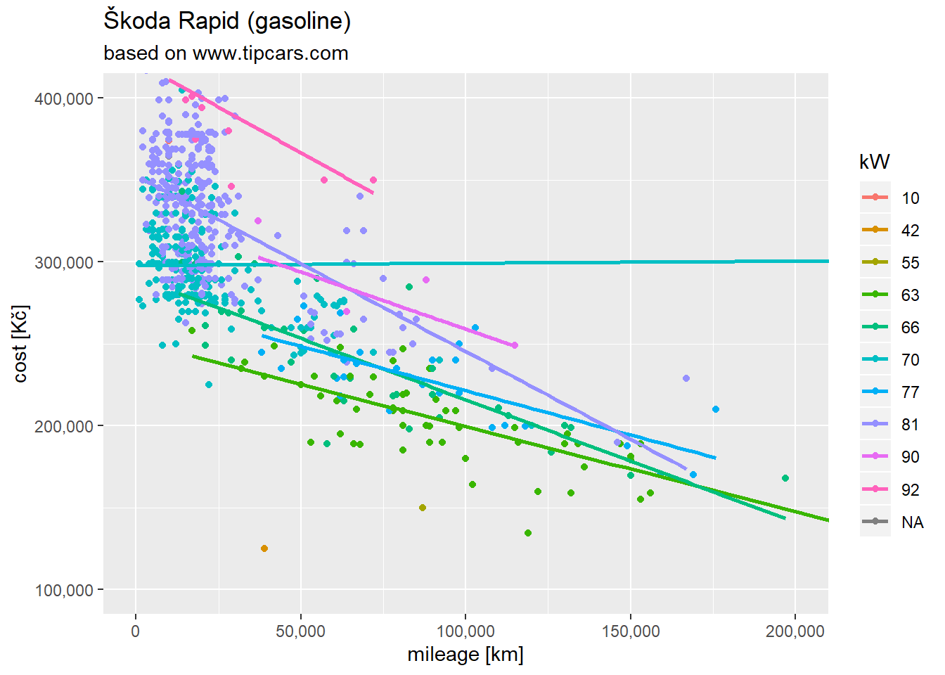
Plot plot plot
final %>%
  ggplot(aes(x = mileage, y = cost, color = kW)) +
  geom_point() +
  scale_x_continuous(labels = comma) +
  scale_y_continuous(labels = comma) +
  coord_cartesian(xlim = c(0,200000), ylim = c(100000, 400000)) +
  geom_smooth(method = "lm", se = FALSE) +
  labs(title = "Škoda Rapid (gasoline)", subtitle = "based on www.tipcars.com", x = "mileage [km]", y = "cost [Kč]")
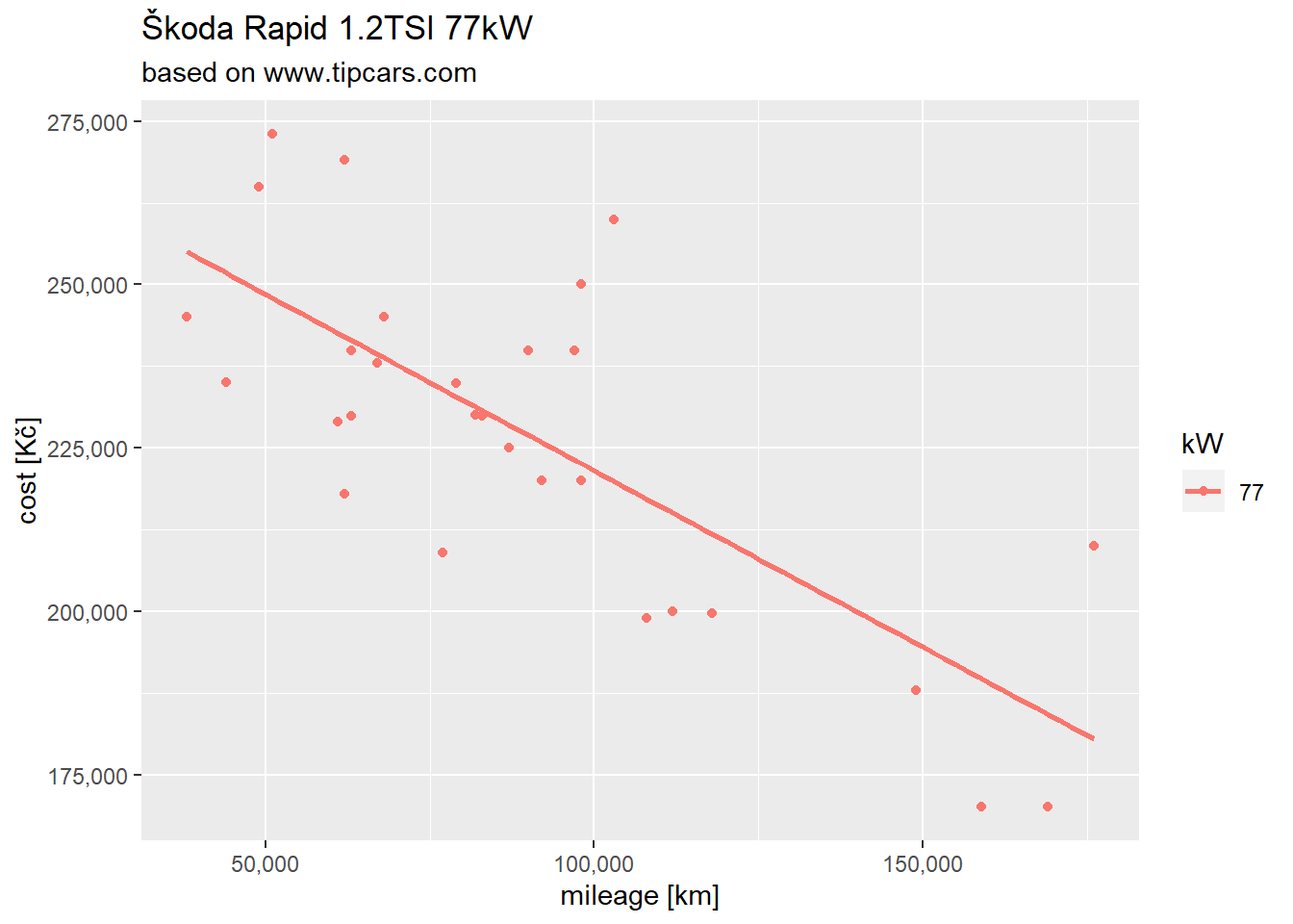
Focused on my car model only:
final %>%
  filter(kW %in% c("77")) %>%

  ggplot(aes(x = mileage, y = cost, color = kW)) +
  geom_point() +
  scale_x_continuous(labels = comma) +
  scale_y_continuous(labels = comma) +
  # coord_cartesian(xlim = c(0,200000), ylim = c(100000, 400000)) +
  geom_smooth(method = "lm", se = FALSE) +
  labs(title = "Škoda Rapid 1.2TSI 77kW", subtitle = "based on www.tipcars.com", x = "mileage [km]", y = "cost [Kč]")
So, what is the value? We need a bit of linear regression..
In order to get single value we have to calculate regression coefficients.
coeff <- final %>%
  filter(kW %in% c("77")) %>%
  lm(cost~mileage, data = .) %>%
  tidy()
coeff
## # A tibble: 2 x 5
## term estimate std.error statistic p.value
## <chr> <dbl> <dbl> <dbl> <dbl>
## 1 (Intercept) 275560. 8747. 31.5 2.07e-23
## 2 mileage -0.540 0.0910 -5.94 2.16e- 6Here we can infer that with each 1km on the road the car looses its value by ~0,5 Kč (~2 Eurocent).
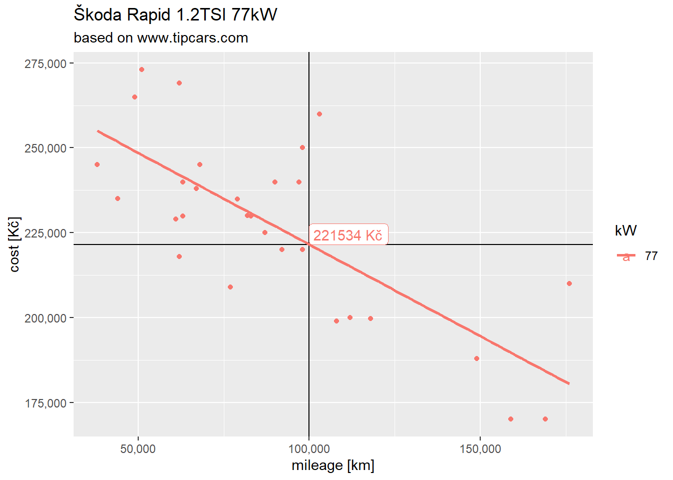
So assuming my car has around 100Tkm mileage its current value is around:
my_mileage = 100000
y = coeff$estimate[1] + (my_mileage * coeff$estimate[2])
paste(round(y), "Kč")
## [1] "221534 Kč"Or visually:
final %>%
  filter(kW %in% c("77")) %>%

  ggplot(aes(x = mileage, y = cost, color = kW)) +
  geom_point() +
  scale_x_continuous(labels = comma) +
  scale_y_continuous(labels = comma) +
  geom_hline(aes(yintercept = y)) +
  geom_vline(aes(xintercept = my_mileage)) +
  geom_label(aes(x = my_mileage, y = y,label = paste(round(y), "Kč")), hjust = 0, vjust = 0) +
  # coord_cartesian(xlim = c(0,200000), ylim = c(100000, 400000)) +
  geom_smooth(method = "lm", se = FALSE) +
  labs(title = "Škoda Rapid 1.2TSI 77kW", subtitle = "based on www.tipcars.com", x = "mileage [km]", y = "cost [Kč]")
Ok, that´s it. Hope you enjoyed:)